Examples
Weighting field of a planar sensor
Example that creates a planar silicon sensor with a given geometry.
Calculates the weighting potential and fields. For comparison also the analytical result of a planar sensor with 100% fill factor (width = pitch) is created.
Note
With increasing distance from the center pixel the numerical result deviates from the analytical one. This shows that is is important to use several pixels (> 5) to get a proper field description in the center pixel.
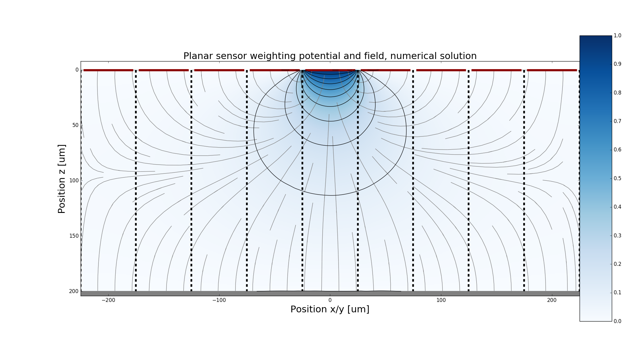
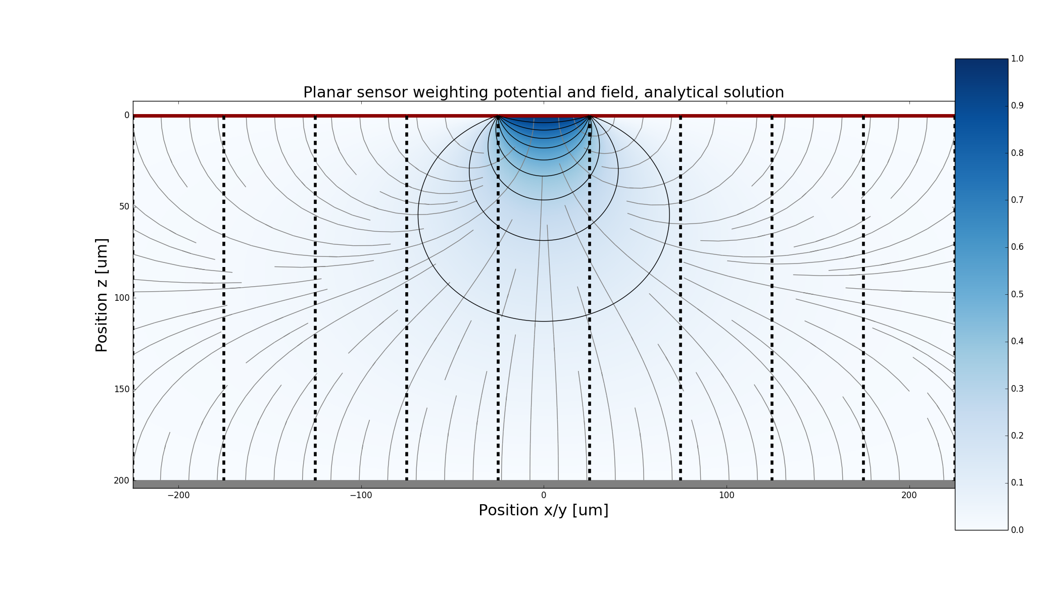

The mesh size determines the quality of the numerical result and can be changed in the example.
Potential of a planar silicon sensor
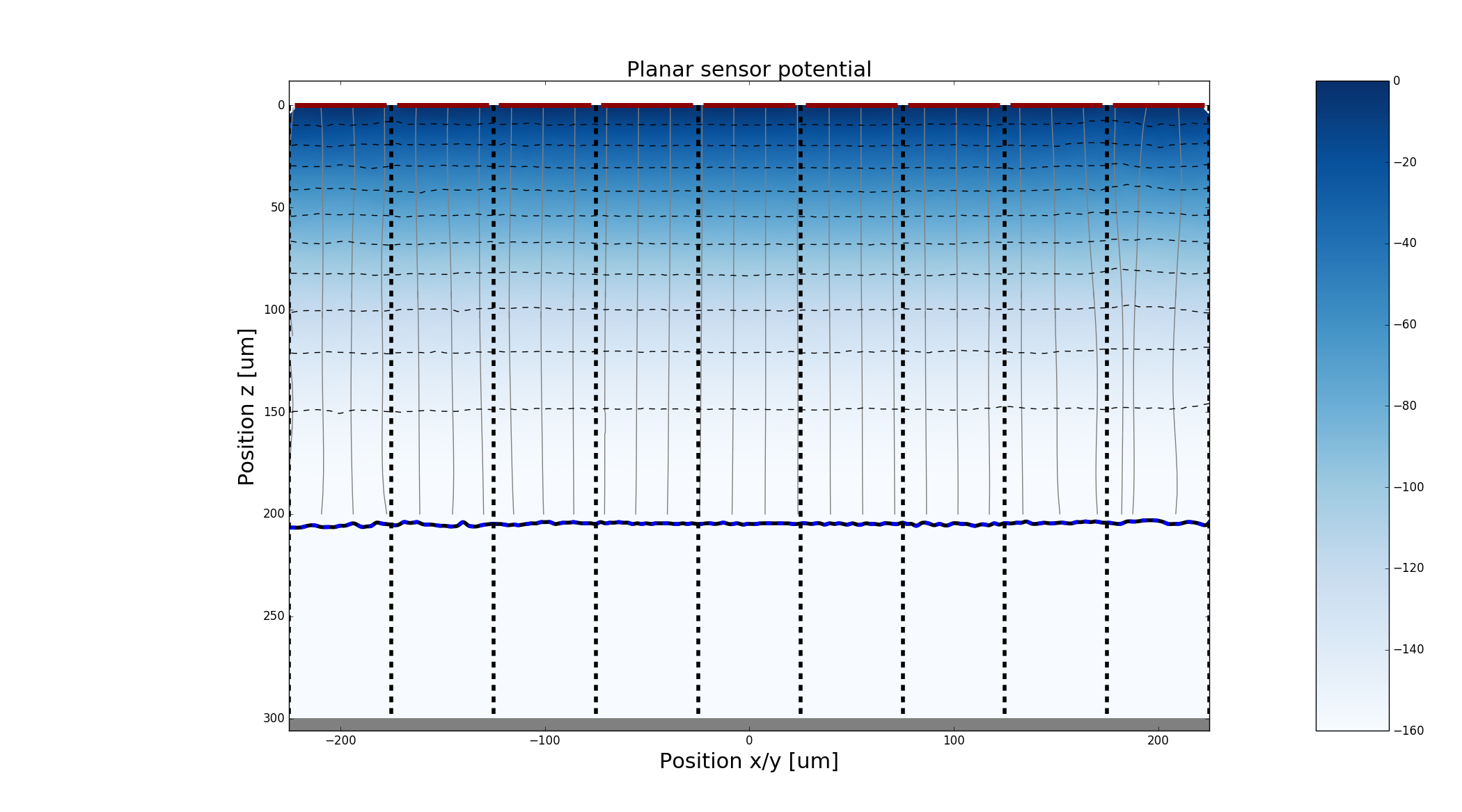
Example that creates a planar silicon sensor with a given geometry.
Calculates the electrical potential and fields. For comparison also the analytical result of a planar sensor with 100% fill factor (width = pitch) is created.
Warning
The calculation of the depletion region is simplified. If the depletion is not at a contant y position in the sensor (e.g. for pixels with very small fill factor) it deviates from the correct solution.
Weighting field of a 3D sensor
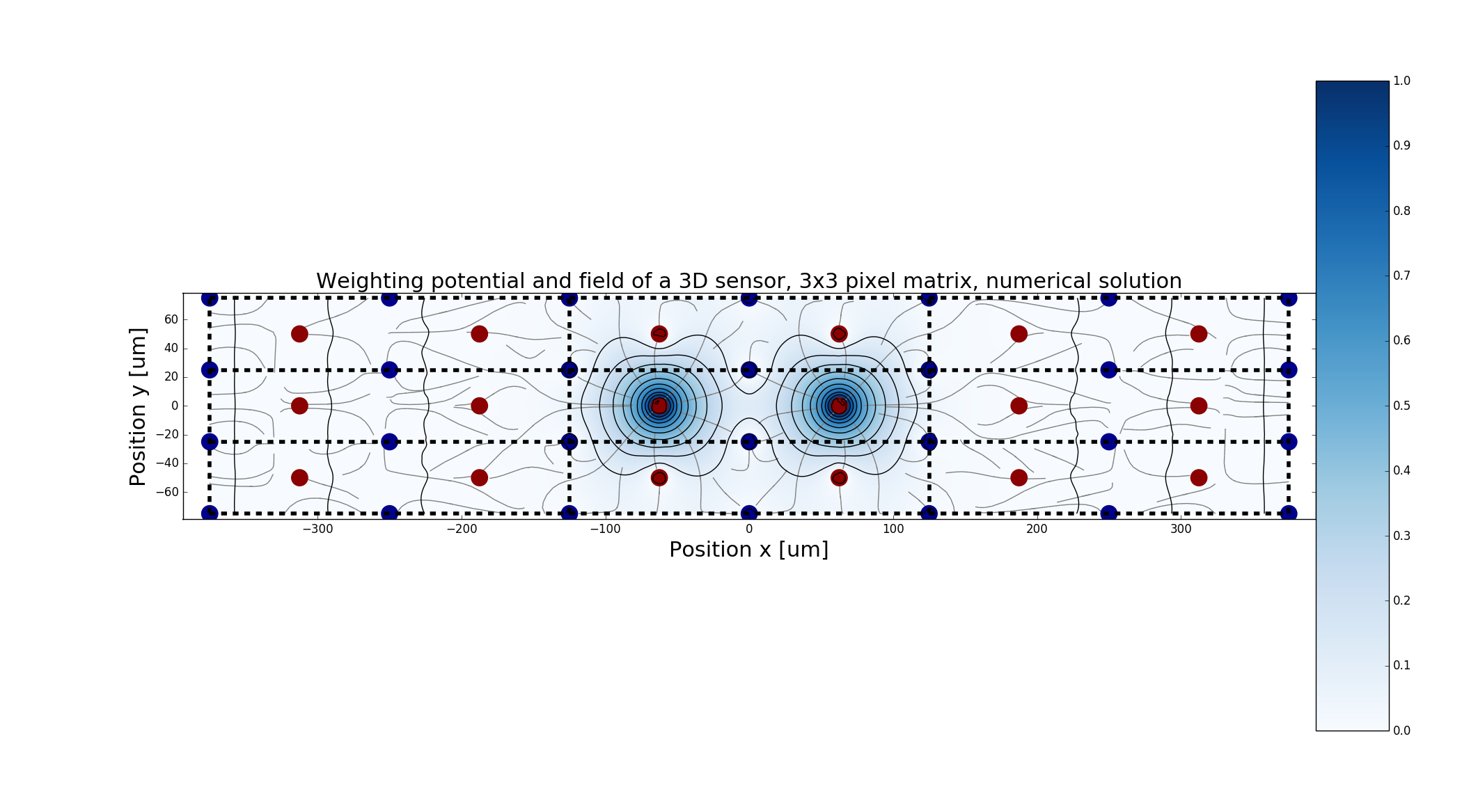
Example creating the weighting field and potential of a 3D pixel array.
Note
The weighting potential and field is only correct if the pixel is surrounded by other pixels, thus n_pixel_x = n_pixel_y = 3
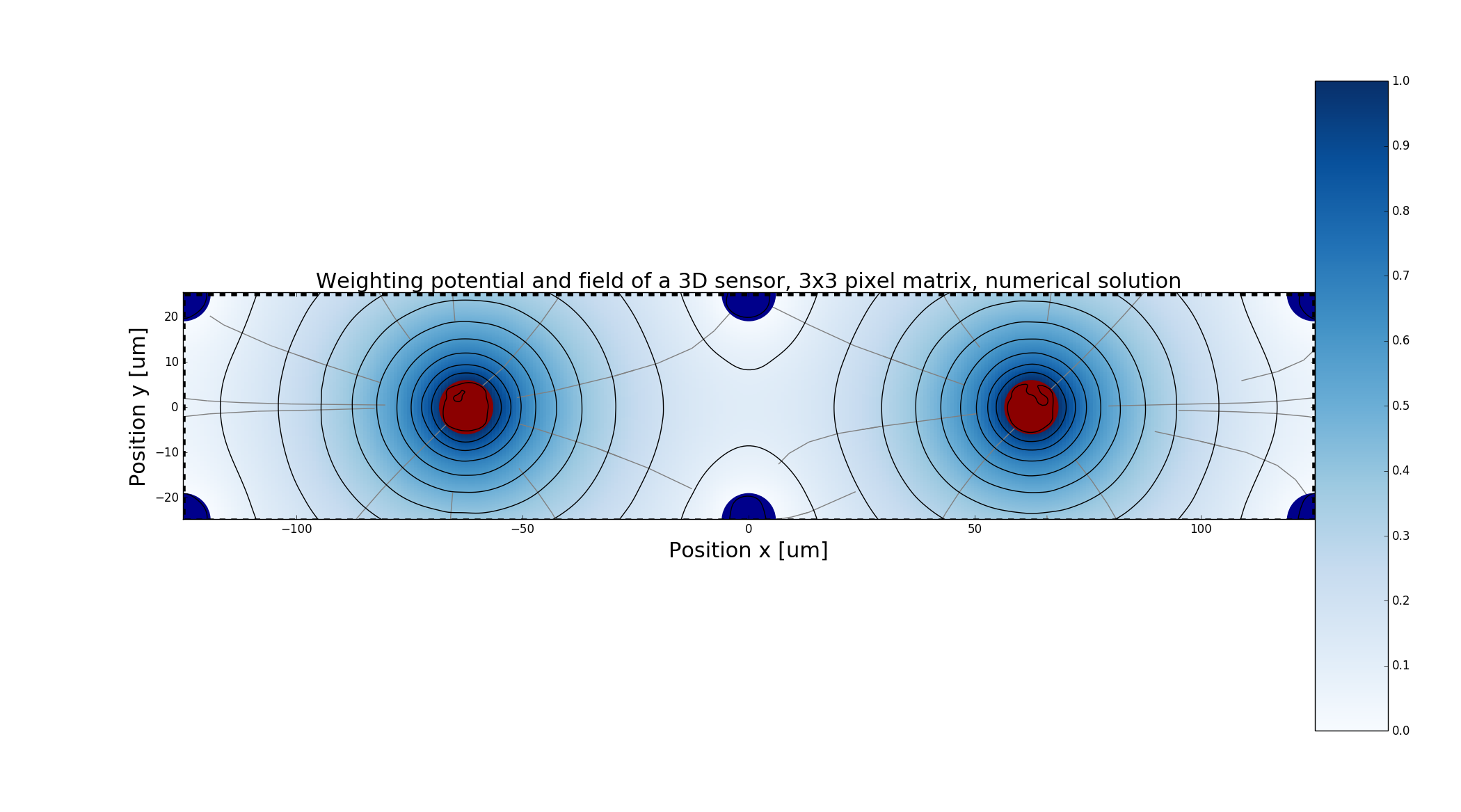
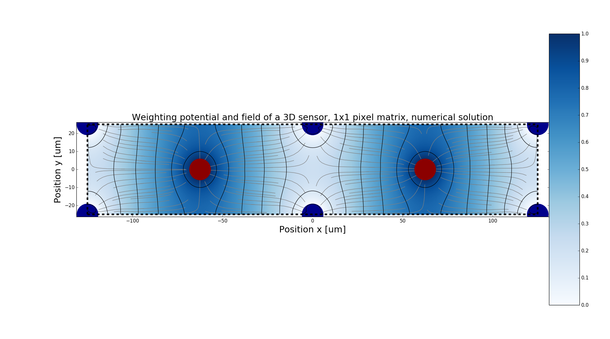
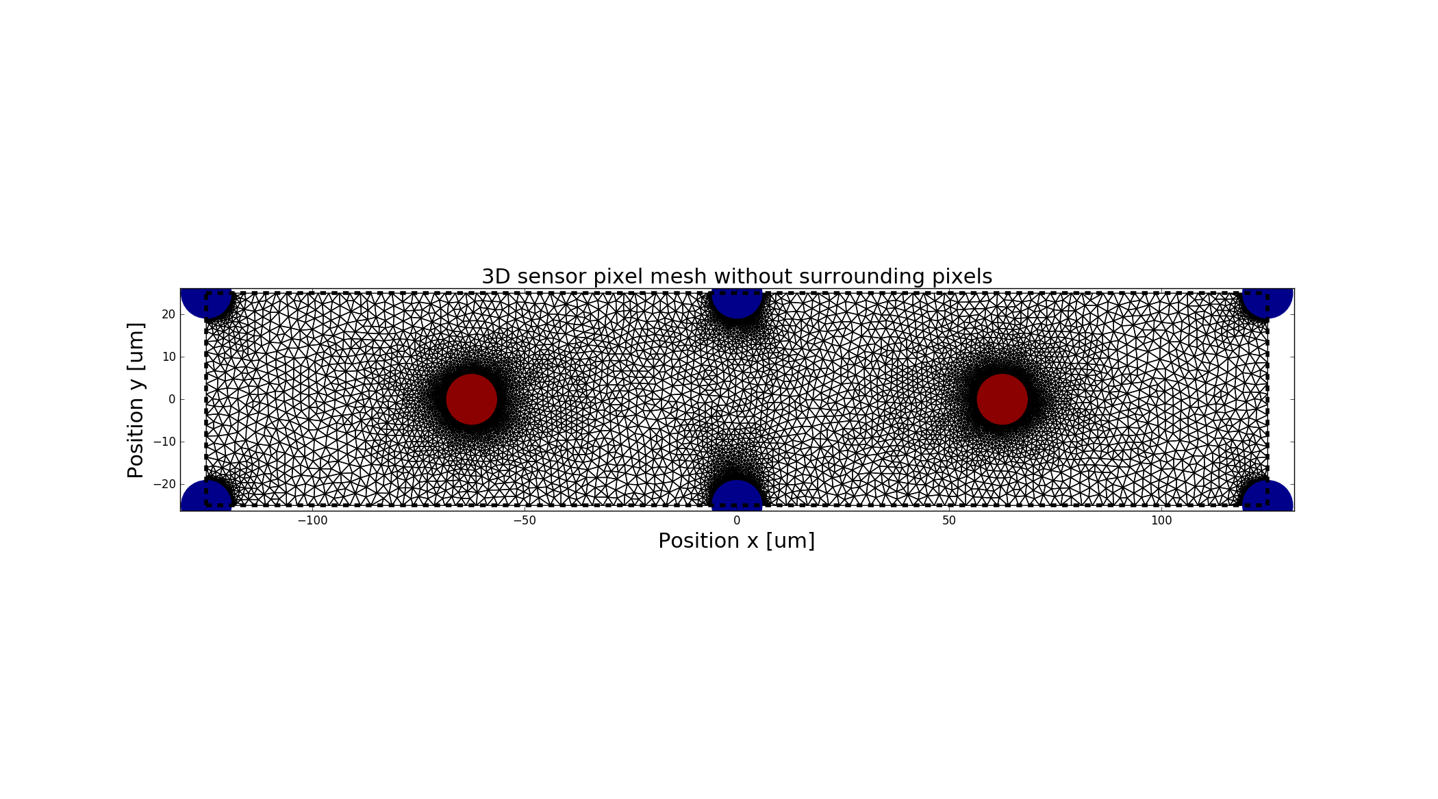
The mesh size determines the quality of the numerical result and can be changed in the example.
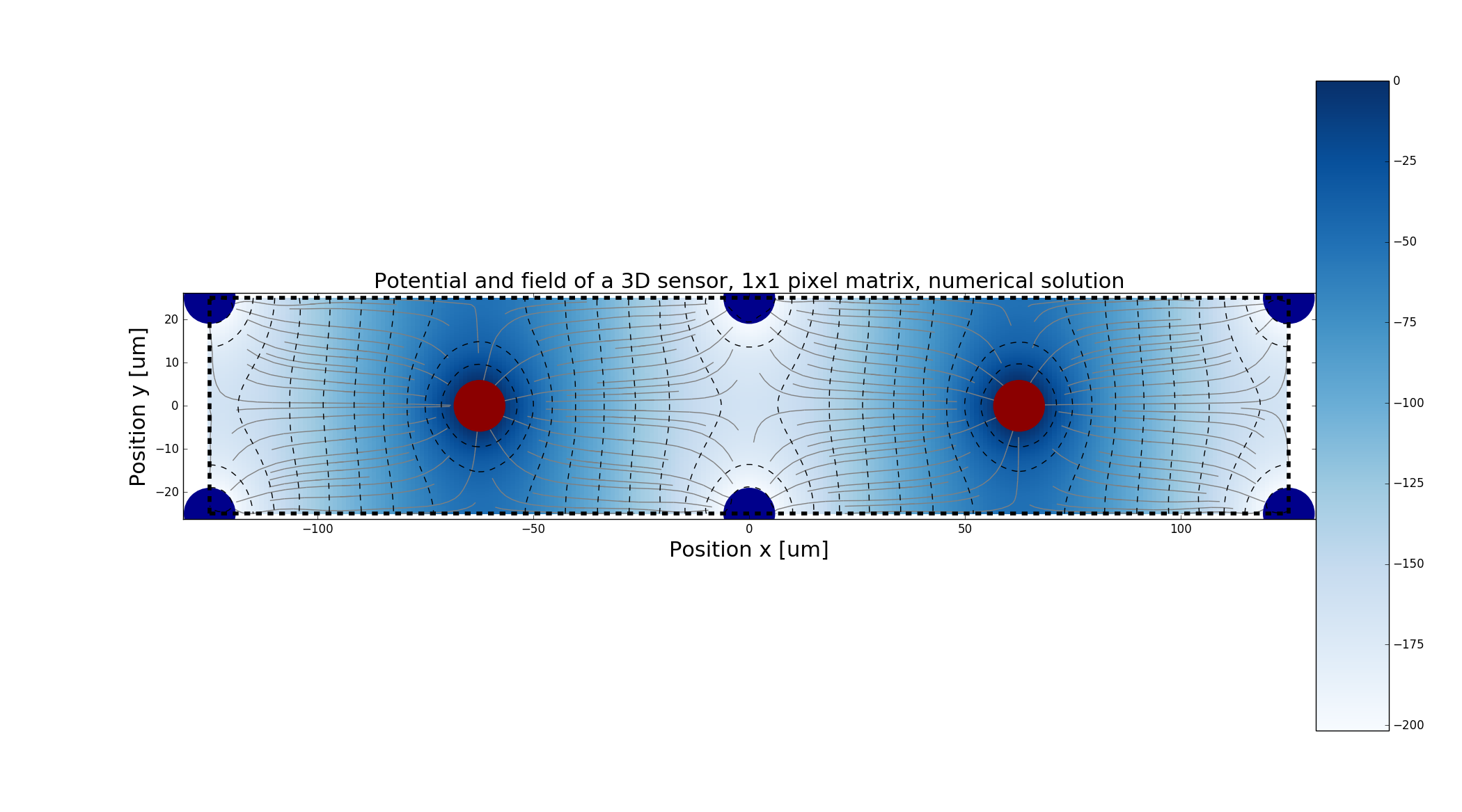
Potential of a 3D sensor
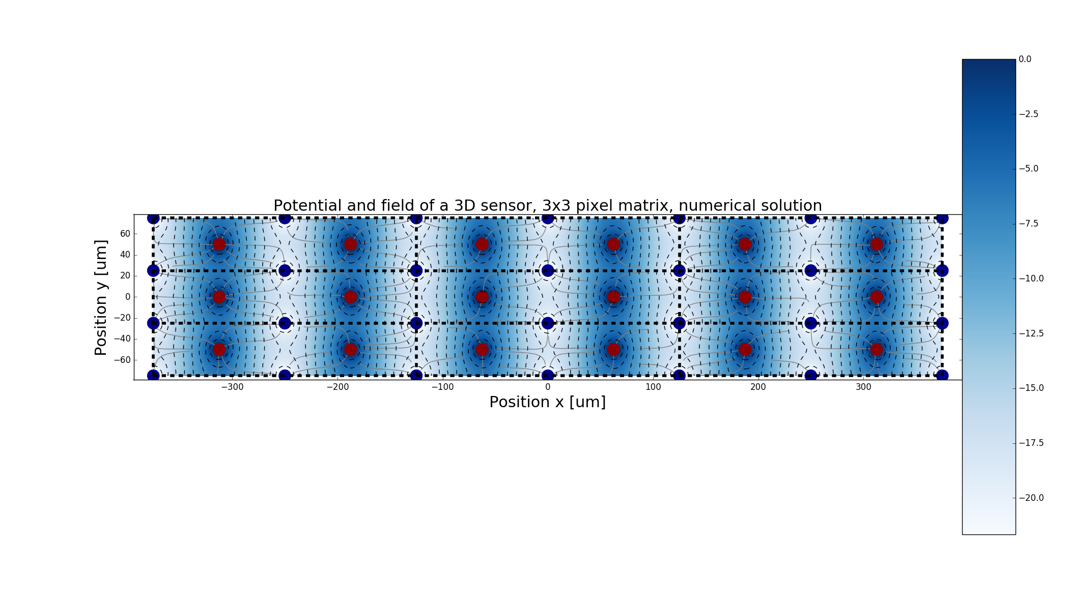
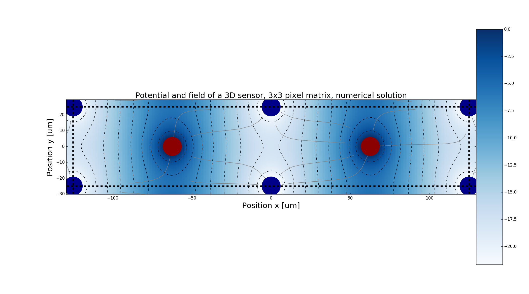
Example that creates a 3D pixel array with a given geometry.
Note
The calculation of a partially depleted 3D sensor is supported.
1D potential in a planar silicon sensor
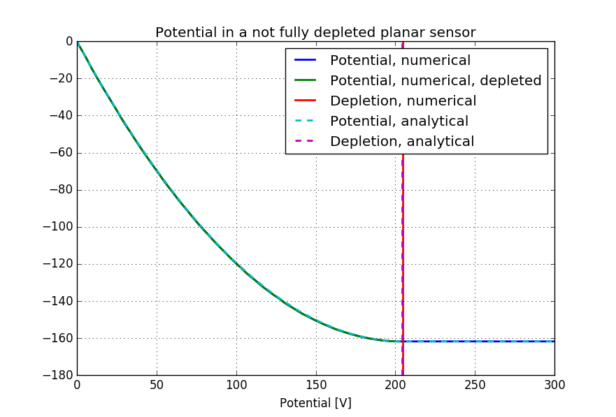
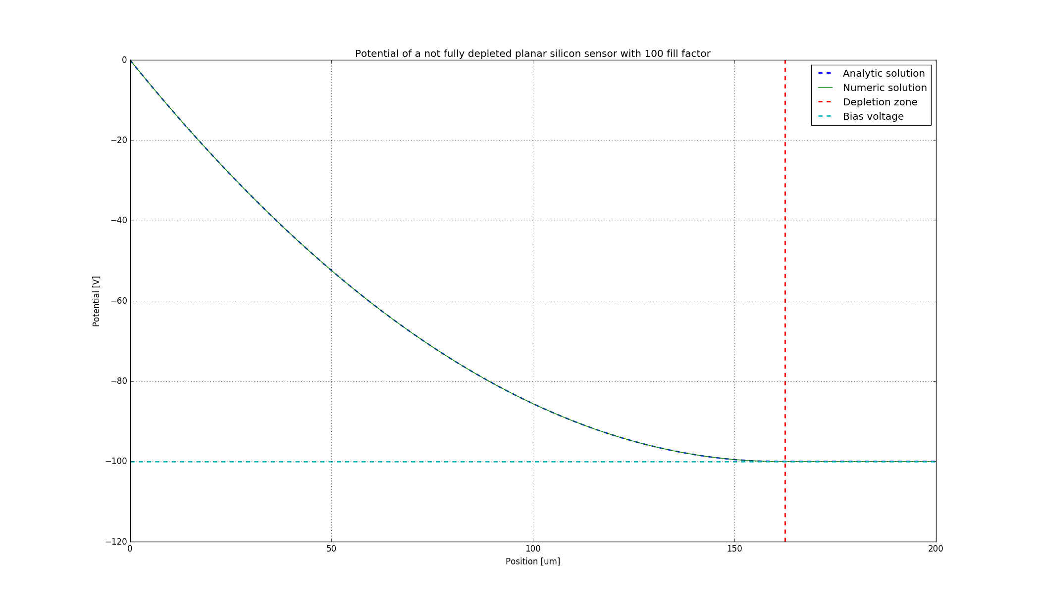
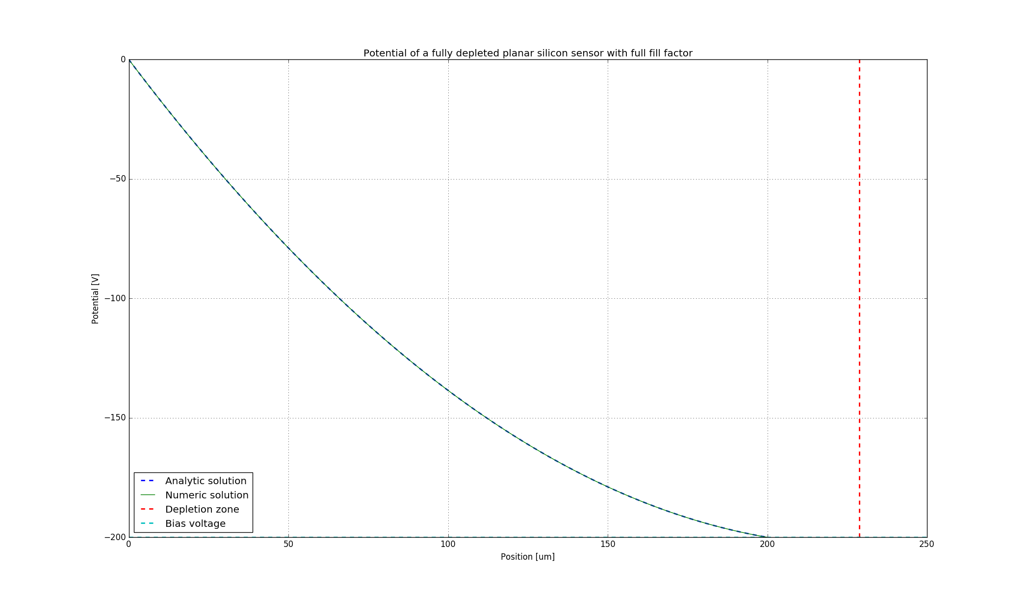
Example that shows the potential in a planar sensor in 1D.
A not fully depleted is supported.The poisson equation is solved numerically and compared to the analytical solution. The 1D solution is also correct in the 2D case for a sensor with 100% fill factor.
The numerical solving for underdepleted sensors is not straight forward, due to the a priory unknown depletion depth. This example shows also how to deal with that.
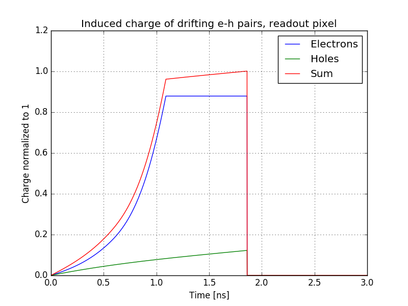
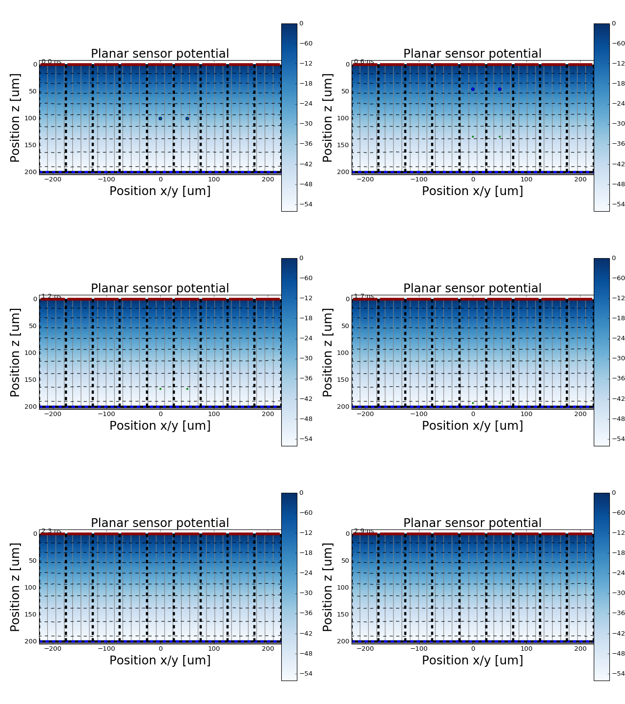
Drifting e-h pairs in planar sensor
Example that moves e-h pairs in a planar sensor.
Calculates the induced charge from e-h pairs drifting through the silicon.
Drifting e-h pairs in 3D sensor
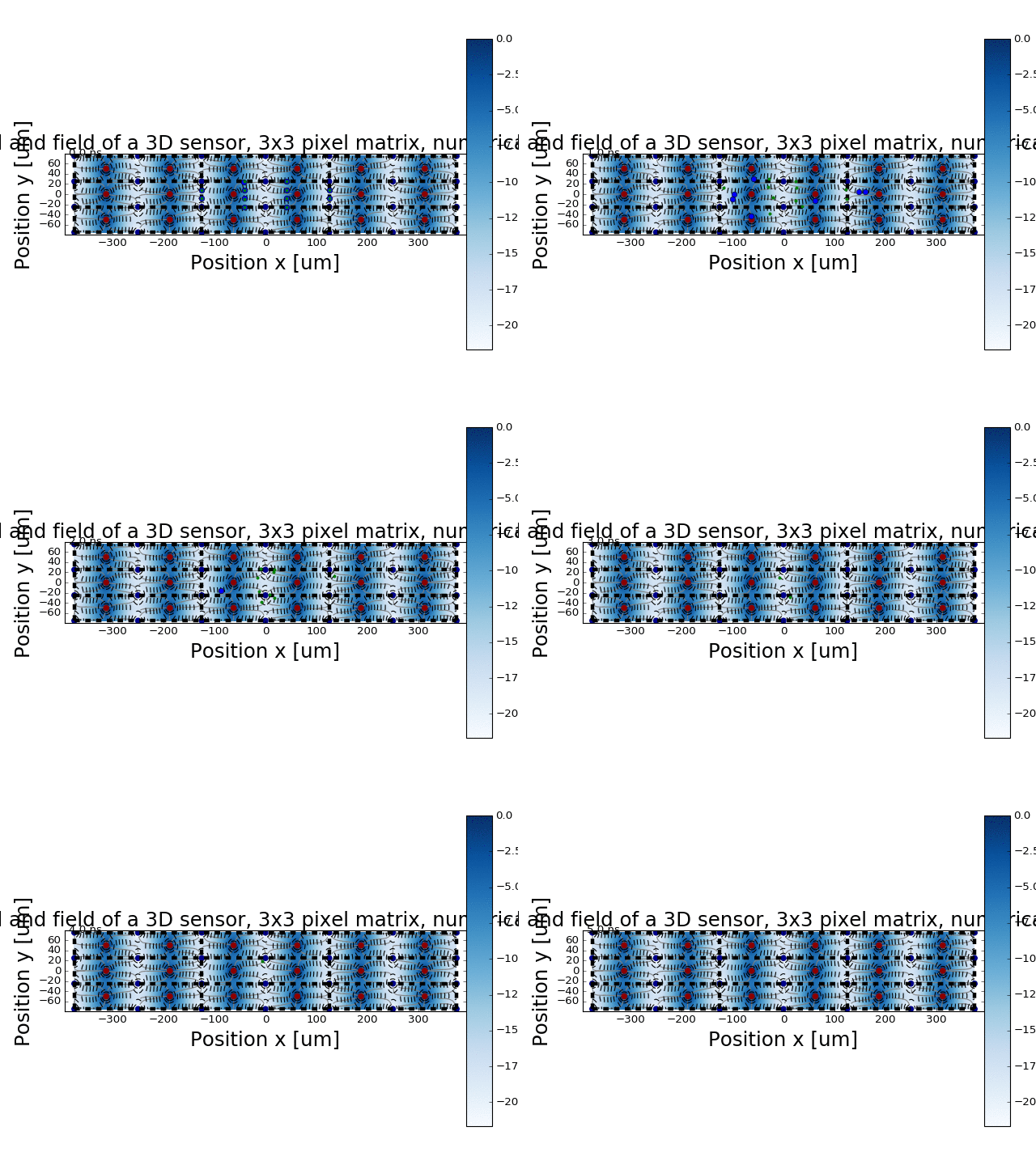
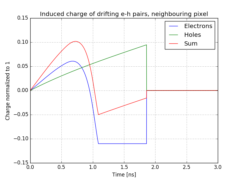
Example that moves e-h pairs in a 3D sensor.
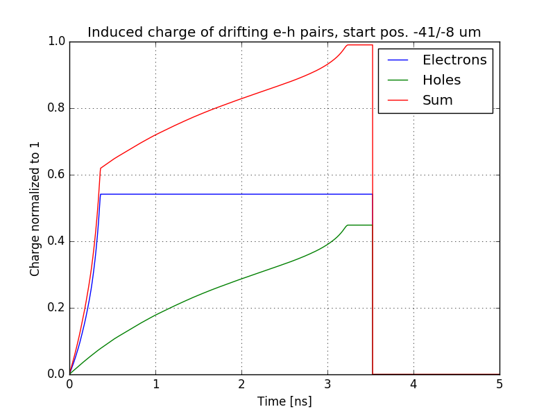
Calculates the induced charge from e-h pairs drifting through the silicon.
Warning
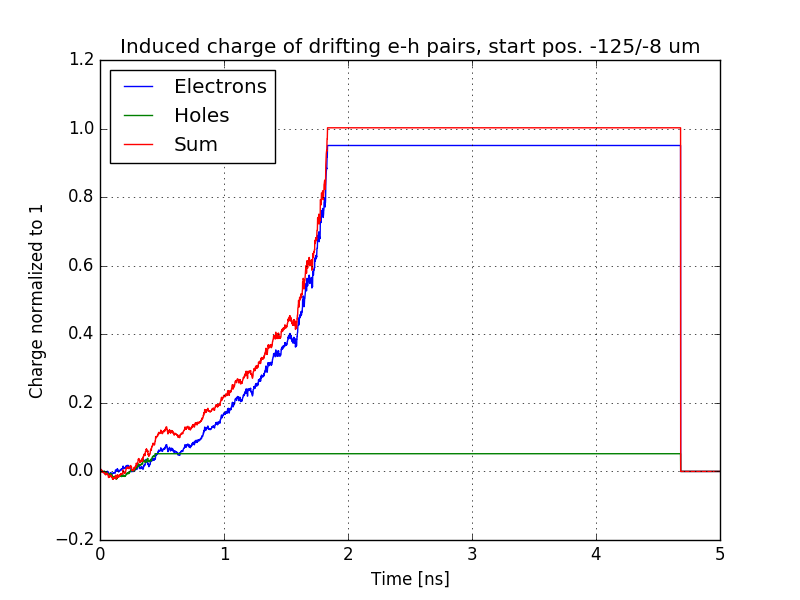
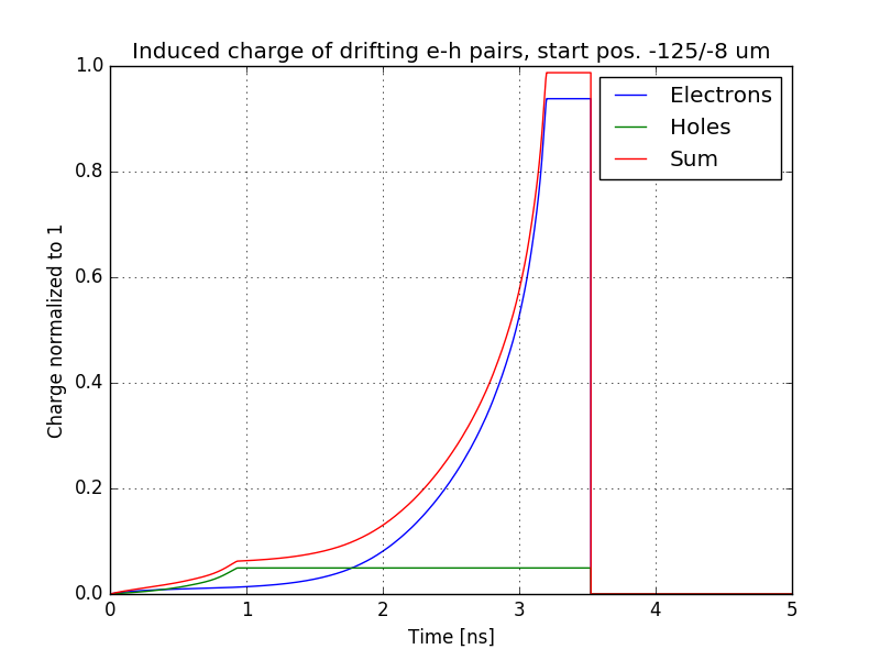
The 3D field is low between pixels. Thus diffusion should be activated to leave this field minima quickly to give reasonable results.
The following shows the induced charge for e-h pairs at different start positions with and without diffusion.
With diffusion:
Without diffusion:
With diffusion:
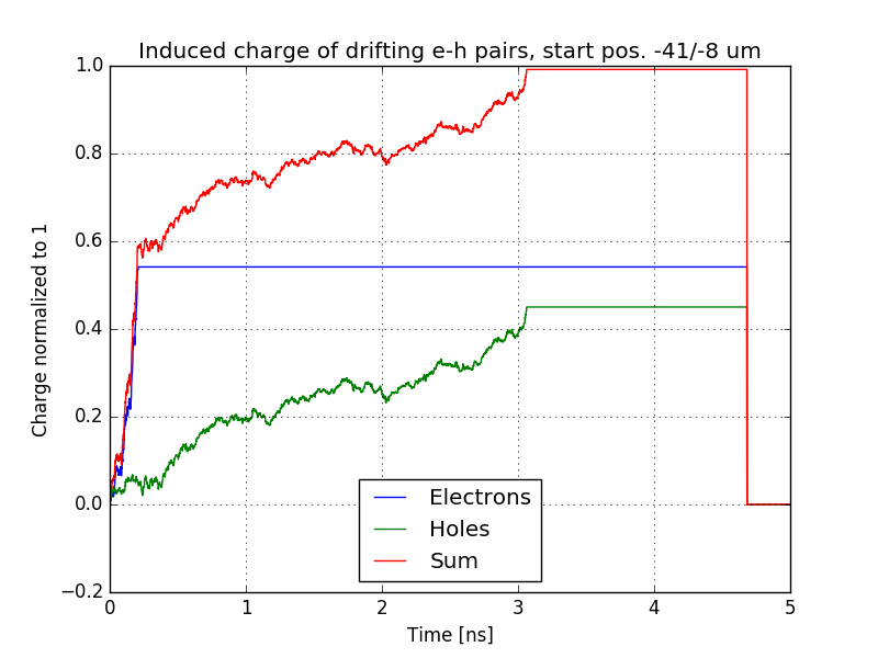
Without diffusion: